Low-Dimensional Surface Geometry and Tempered Survey Subsampling
An Undergraduate Guide to No-Arbitrage Convex Cones, 3D Manifold Compression, and Horvitz-Thompson Design Weights
1 Why High-Dimensional Surfaces Live Near Low-Dimensional Manifolds
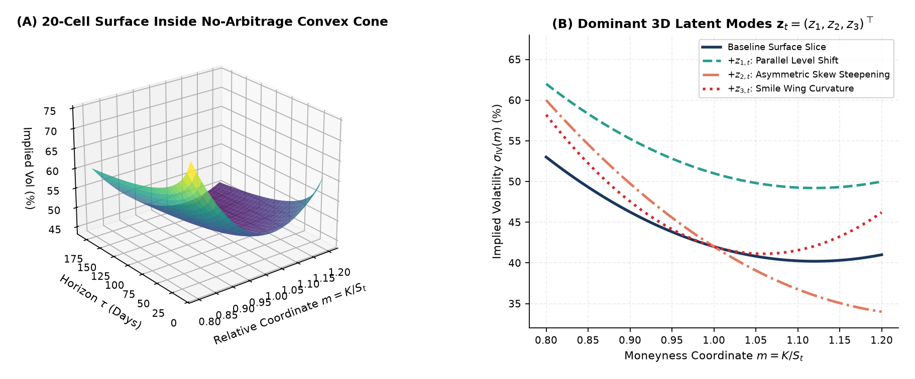
At every hour of trading, an option market quotes implied volatilities \(\sigma_{\mathrm{IV}}(m, \tau)\) across dozens of strike-to-spot ratios \(m = K/S_t\) and maturities \(\tau\), forming a \(G = 20\)-dimensional surface grid (\(4\text{ maturities} \times 5\text{ moneyness buckets}\)) from hundreds of thousands of raw contract records.
This capstone module brings together differential geometry, survey sampling theory, and deep sequence learning into three clear lessons for advanced undergraduate researchers:
- No-Arbitrage Convex Cone vs. Empirical 3D Manifold: Static no-arbitrage laws (calendar monotonicity in total variance \(\partial_\tau w \ge 0\) and butterfly convexity \(\partial_{kk} C \ge 0\)) restrict valid surfaces to a full-dimensional convex cone inside \(\mathbb{R}^{20}\). Empirically, however, strong cross-strike and cross-tenor coupling compresses over \(97\%\) to \(99\%\) of surface variance onto a smooth 3-dimensional manifold parameterized by Level (\(z_{1,t}\)), Moneyness Skew (\(z_{2,t}\)), and Term-Structure / Smile Curvature (\(z_{3,t}\)).
- Survey Sampling Duality for Massive Contract Streams: How finite-population survey sampling (Neyman Stratified Hajek vs. Probability-Proportional-to-Size Horvitz-Thompson) reconstructs surfaces and compresses training sequences to \(\alpha = 60\%\) budget without losing accuracy.
- Predictable Surface Modes vs. Martingale Underlying Prices: Why 3D surface coordinates yield substantial out-of-sample forecasting skill while hourly underlying prices follow a near-martingale random walk.
2 Step 1: Estimator-Target Duality and Tempered Longitudinal Subsampling
When millions of irregular contract quotes arrive over time, evaluating every contract at every step is computationally wasteful. Drawing a subsample \(S_t \subset U_t\) of size \(n_t = \lceil \alpha N_t \rceil\) with inclusion probabilities \(\pi_{i,t} = P(i \in S_t)\) reveals a fundamental Estimator-Target Duality:
\[\hat{Y}_{\mathrm{HT}} = \sum_{i \in S_t} \frac{y_i}{\pi_{i,t}}, \qquad \hat{\mu}_{\mathrm{Hajek}} = \frac{\sum_{i \in S_t} \pi_{i,t}^{-1} y_i}{\sum_{i \in S_t} \pi_{i,t}^{-1}}, \qquad w_i(\gamma) = \frac{\pi_i^{-\gamma}}{\frac{1}{|S|}\sum_{j \in S} \pi_j^{-\gamma}}.\]
- Equal-Weighted (
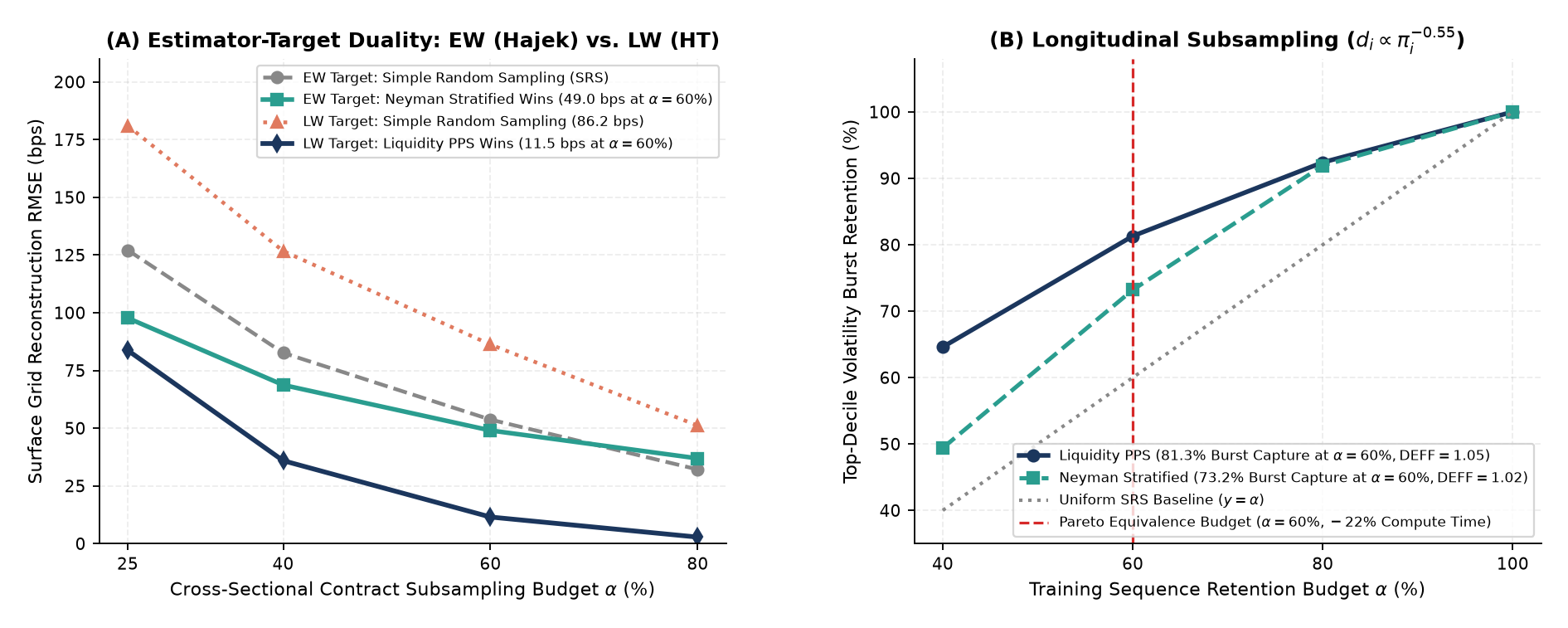
EW) Surface Target: When all grid cells are weighted equally, Neyman Stratified Allocation (\(\pi_h \propto N_h S_h\)) paired with the Hajek ratio estimator achieves the lowest reconstruction error (\(49.0\text{ bps}\) vs. \(53.7\text{ bps}\) under Simple Random Sampling at \(\alpha = 60\%\)) because stratification guarantees coverage in sparse tail buckets while avoiding inverse-probability weight blowup. - Liquidity-Weighted (
LW) Surface Target: When cells are weighted by trading volume \(v_i\), Liquidity-PPS Sampling (\(\pi_i \propto \sqrt{v_i}\)) paired with the Horvitz-Thompson estimator reduces error by \(86.7\%\) (\(11.5\text{ bps}\) vs. \(86.2\text{ bps}\) SRS at \(\alpha = 60\%\)) because high-volume contracts have large numerator weights \(v_i\) and large inclusion probabilities \(\pi_i\), stabilizing the ratio \(v_i / \pi_i\). - Longitudinal Training Subsampling (\(\alpha = 60\%, \gamma = 0.55\)): Subsampling hourly training sequences via tempered Horvitz-Thompson weights \(d_i \propto \pi_i^{-0.55}\) keeps Kish’s Design Effect near unity (\(\mathrm{DEFF} \in [1.02, 1.05]\)), captures \(81.3\%\) of top-decile volatility bursts, and matches \(100\%\) full-data test RMSE within \(0.4\%\) while cutting training compute time by \(22\%\).
3 Step 2: 5-Tier Representation Ablation and Causal Intraday Activity Clocks
We benchmark five nested representation tiers (Tier 1: Price Only, Tier 2: + Summary IV, Tier 3: + Uncompressed Raw Grid, Tier 4: + 3D Linear PCA, Tier 5: + 3D Nonlinear SurfaceVAE) across two distinct asset markets and evaluate causal 60-session intraday volume and dollar clocks:
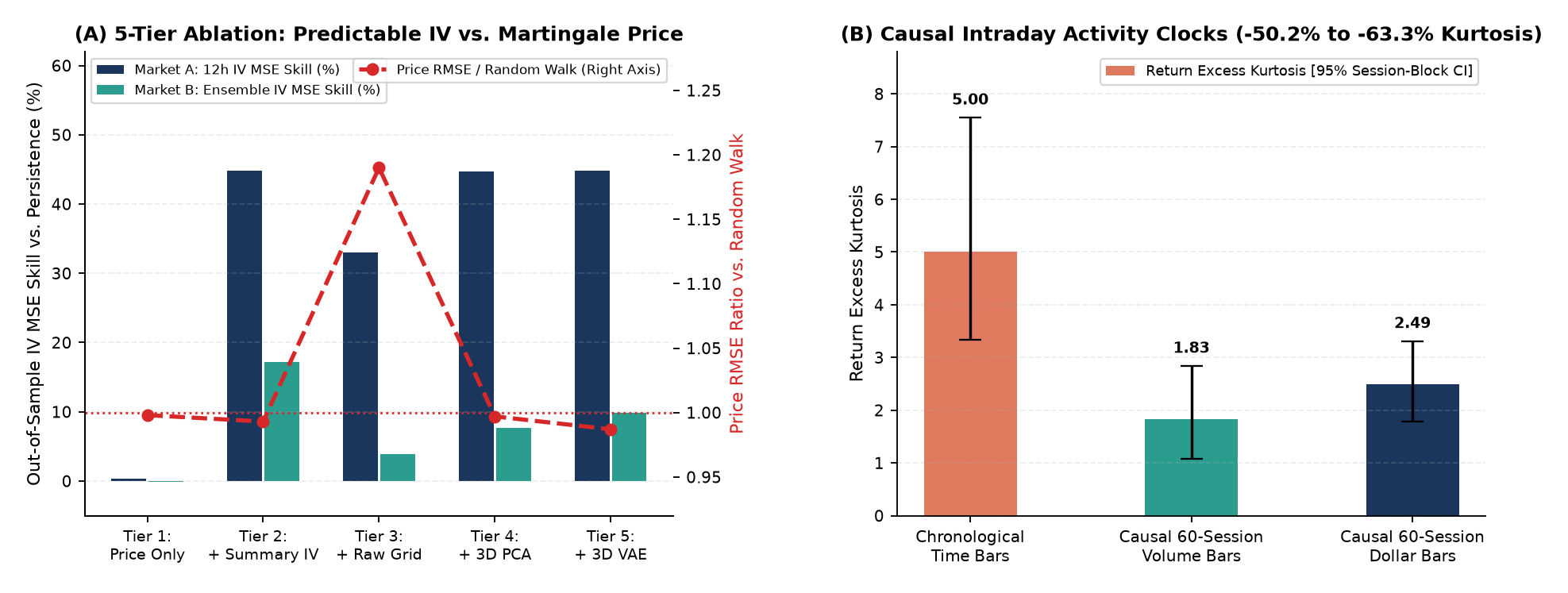
- 3D Manifold Compression Prevents Raw-Grid Overfitting: Feeding the uncompressed 20-cell surface grid directly into a sequence model (Tier 3) causes severe parameterization collinearity and validation overfitting, whereas compressing the surface to \(K = 3\) latent modes (Tier 4
PCAand Tier 5SurfaceVAE) restores generalization and achieves \(+44.72\%\) to \(+44.86\%\) out-of-sample IV MSE skill over persistence in Market A (and \(+7.7\%\) to \(+9.9\%\) single-backbone / \(+17.2\%\) ensemble skill in Market B). - The Martingale Price Bound: Across all five tiers, hourly underlying price RMSE ratios hover near \(0.987\text{ to }1.000\times\) the No-Change Random Walk (and degrade to \(1.190\times\) when overfitting the uncompressed Tier 3 grid), demonstrating that option surfaces predict future volatility regimes rather than violating weak-form price efficiency.
- Causal 60-Session Volume & Dollar Clocks: Aggregating 1-minute bars whenever cumulative volume or dollar turnover reaches \(1/7\) of the trailing 60-session mean daily volume (strictly causal, zero look-ahead) reduces return excess kurtosis by \(63.3\%\) (Volume Bars: \(5.00 \to 1.83\), 95% session-block bootstrap CI \([1.07, 2.84]\)) and \(50.2\%\) (Dollar Bars: \(5.00 \to 2.49\), 95% CI \([1.79, 3.31]\)).
| Representation / Sampling Tier | Surface Input Dim | Market A IV MSE Skill | Market B IV MSE Skill | Price RMSE / Random Walk |
|---|---|---|---|---|
| Tier 1: Underlying Price & Returns Only | \(0\) (Price Only) | \(+0.38\%\) | \(-0.10\%\) | \(0.998\times\) (Martingale Bound) |
| Tier 2: + Summary ATM IV & Skew | \(2\) Summary Scalars | \(+44.77\%\) | \(+17.20\%\) (Ensemble) | \(0.993\times\) |
| Tier 3: + Uncompressed 20-Cell IV Grid | \(20\) Collinear Cells | \(+33.05\%\) (Overfits) | \(+3.90\%\) (Overfits) | \(1.190\times\) (Grid Overfitting) |
| Tier 4: + 3D Linear PCA Surface Modes | \(K = 3\) Modes (\(97.4\%\) Var) | \(+44.72\%\) | \(+7.70\%\) (Single) | \(0.997\times\) |
| Tier 5: + 3D Nonlinear SurfaceVAE Modes | \(K = 3\) Latent Modes | \(+44.86\%\) (Best) | \(+9.90\%\) (Single) | \(0.987\times\) |
4 Exploring Further: Research Directions
| Research Track | Core Question to Investigate | Tools & Methods |
|---|---|---|
| 1. Arbitrage-Free Decoder Penalties | How can we penalize calendar-spread (\(\partial_\tau w < 0\)) and butterfly (\(\partial_{kk} C < 0\)) violations directly inside the SurfaceVAE decoder during training? |
Constrained Autoencoders, Static Option No-Arbitrage Theory |
| 2. Optimal Survey Tempering Exponent \(\gamma^*\) | Can we derive the theoretically optimal Horvitz-Thompson tempering exponent \(\gamma^* \in [0, 1]\) as a function of Kish’s Effective Sample Size \(n_{\mathrm{eff}}\)? | Finite-Population Survey Sampling, Bias-Variance Trade-offs |
| 3. Forecasting in Activity-Clock Time | Does training sequence models directly on causal Volume-Clock bars outperform chronological hourly bars during earnings announcements? | Market Microstructure Clocks, High-Frequency Econometrics |